

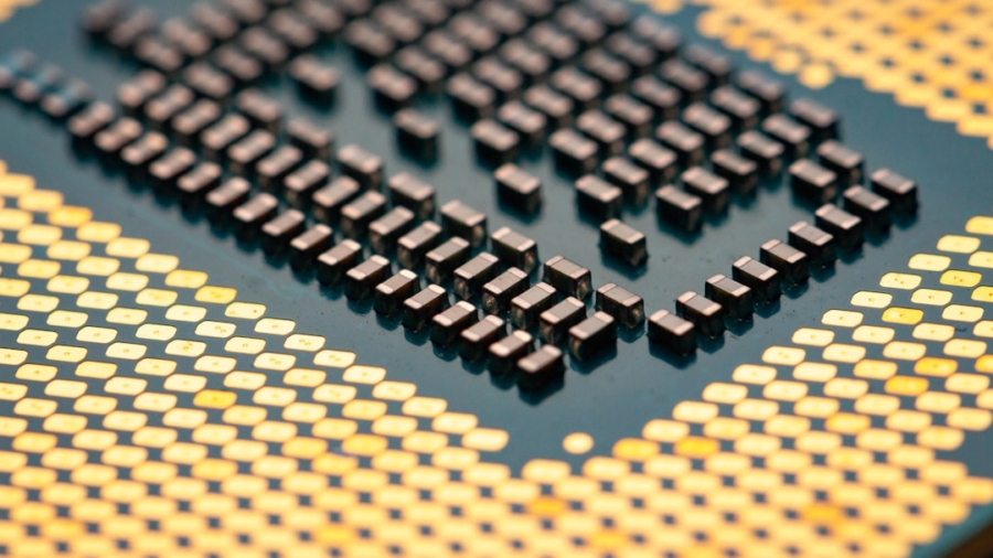
When we talk about making AI, specifically deep learning, more efficient, one of the most exciting areas right now is Analog In-Memory Computing (AIMC). Put simply, it’s about doing computations directly within the memory, rather than constantly moving data back and forth between separate processing units and memory banks. This approach tackles a fundamental bottleneck in traditional computer architectures, known as the “von Neumann bottleneck,” where data transfer consumes a huge amount of energy and time. AIMC promises to drastically reduce the energy consumption and speed up inference for deep learning models, making AI more accessible and practical for everything from edge devices to large data centers.
Why Traditional Computing Struggles with AI
Before diving into AIMC, it’s helpful to understand why current systems aren’t ideal for AI.
The Von Neumann Bottleneck Explained
Imagine you’re trying to bake a cake. In a traditional computer, your recipe (the instructions) is in one room, and your ingredients (the data) are in another. Every time you need an ingredient or need to check a step, you have to run back and forth. This constant running around is what we call the von Neumann bottleneck. For deep learning, which involves billions of multiplications and additions on huge datasets, this “running around” for data transfer dominates energy consumption and slows everything down.
Energy and Latency Costs of Data Movement
Think about it: moving a single bit of data from a memory module to a processor core can consume hundreds or even thousands of times more energy than performing a simple arithmetic operation on that bit once it’s in the processor. When you’re dealing with gigabytes of neural network weights and activations, these energy costs add up massively. Latency, the time it takes to complete an operation, also suffers significantly because of this data shuttling.
In the realm of optimizing hardware for deep learning inference, the article on how to choose a PC for students offers valuable insights into selecting energy-efficient components that can enhance computational performance. By understanding the requirements for deep learning tasks, students can make informed decisions about their hardware, ensuring that they are equipped with the right tools for their studies. For more information on selecting the best PC for academic purposes, you can read the article here: How to Choose a PC for Students.
The Core Idea Behind Analog In-Memory Computing
AIMC offers a fresh perspective by bringing computation closer to the data, effectively trying to bake the cake right where the ingredients are stored.
Merging Memory and Computation
Instead of a clear separation, AIMC integrates computational capabilities directly into memory devices. This means that when you store a neural network’s weights in an AIMC array, you can also perform the necessary multiplications and additions within that very same array. This significantly cuts down on the need to move data to a separate processing unit, thereby sidestepping the von Neumann bottleneck.
Leveraging Analog Principles
The “analog” part is key here. Unlike digital computing, which represents data as discrete 0s and 1s, analog computing uses continuous physical quantities like voltage or current to represent data. In AIMC, this often involves using physical properties of memory elements, like resistance, to perform computations. For instance, Ohm’s law (V=IR) can be directly exploited: if you represent one number as current and another as resistance, the resulting voltage can represent their product. Summing these voltages can then perform the accumulation step vital for neural network operations. This direct physical implementation can be much more energy-efficient than converting everything to digital, processing it, and then converting it back.
Key Technologies for Analog In-Memory Computing
Several memory technologies are being explored for AIMC, each with its own strengths and challenges.
Resistive Random Access Memory (RRAM/ReRAM)
RRAM is a front-runner for AIMC. It’s a type of non-volatile memory where the resistance of a material can be controllably changed and maintained, even without power.
How RRAM Works for AIMC
In an RRAM crossbar array, individual memory cells (RRAM devices) are placed at the intersections of word lines and bit lines.
The resistance of each cell can be programmed to represent a synaptic weight.
To perform a vector-matrix multiplication – the core operation in neural networks – input voltages representing activations are applied to the word lines. According to Ohm’s law, currents flow through the RRAM cells proportional to the input voltage and the cell’s conductance (which is the inverse of resistance, representing the weight). By summing the currents along the bit lines (Kirchhoff’s current law), you get the output, which is the sum of products. This happens in parallel across the entire array, leading to very high throughput.
Advantages and Challenges of RRAM
Advantages:
- High Density: RRAM cells can be very small, allowing for dense arrays.
- Non-Volatile: Weights are retained even when power is off, which is crucial for edge devices.
- Fast Operation: Computations happen in situ and in parallel.
- Low Power: Significantly reduces data movement power.
Challenges:
- Device Variability: The resistance of RRAM cells can vary significantly from device to device and over time, leading to inaccuracies.
- Limited Endurance: Repeated programming (weight updates during training) can degrade the RRAM cells, limiting their lifespan. This is less of an issue for inference-only systems but still needs consideration for retraining.
- Non-Linearity: The relationship between programming voltage/current and resistance change can be non-linear, making precise weight programming difficult.
- Analog Noise: Being analog, RRAM-based computations are susceptible to various noise sources.
Phase-Change Memory (PCM)
PCM is another non-volatile memory technology based on the reversible phase change of chalcogenide glass between amorphous (high resistance) and crystalline (low resistance) states.
PCM in AIMC Architectures
Similar to RRAM, PCM cells can be arranged in crossbar arrays. The different resistance states can store synaptic weights. By applying appropriate voltage pulses, the phase of the material changes, altering its resistance. The computation proceeds similarly to RRAM, with input voltages, current flow through the programmed resistances, and current summation.
Pros and Cons of PCM
Pros:
- Multi-Level Storage: PCM can often store more than just two distinct resistance states, potentially allowing for higher precision weights per cell.
- Relatively Good Endurance: Generally better than RRAM for many cycles, though still a concern for training.
- Non-Volatile: Like RRAM, weights are retained.
Cons:
- Higher Power Consumption during Programming: Changing the phase typically requires significant current pulses, which can be power-intensive during programming.
- Thermal Cross-Talk: Heating one cell to change its phase can inadvertently affect neighboring cells.
- Resistance Drift: The resistance of the amorphous state can slowly change over time, leading to weight inaccuracies.
Flash Memory
While primarily known for digital storage in SSDs and USB drives, some researchers are exploring Flash memory for AIMC, particularly its multi-level cell (MLC) capabilities.
Flash Memory’s Role in AIMC
Flash cells store charge on a floating gate, which affects the transistor’s threshold voltage and thus its conductance. By carefully controlling the amount of charge, multiple distinct conductance levels can be stored in a single cell, representing different synaptic weights. The “memory” aspect of in-memory computing is inherently present in Flash.
Advantages and Limitations of Flash for AIMC
Advantages:
- Mature Technology: Flash is a highly mature and widely manufactured technology, meaning existing fabrication processes could potentially be adapted.
- High Density: Can achieve very high storage densities.
- Multi-Level Cell (MLC) Potential: Good for storing multiple bits per cell.
Limitations:
- Slow Programming/Erasure: Writing and erasing Flash cells is relatively slow compared to RRAM or PCM, which limits its utility for on-chip learning or frequent weight updates.
- Limited Endurance: Similar to other non-volatile memories, Flash has a finite number of program/erase cycles.
- Read Disturb: Reading one cell can sometimes inadvertently affect the charge stored in neighboring cells.
- Analog Readout Challenges: Extracting precise analog values from Flash cells for computation in an analog domain can be complex.
Designing AIMC Systems: Beyond the Memory Cell
An effective AIMC system is more than just a fancy memory cell; it requires a holistic approach to design.
Peripheral Circuitry: The Unsung Heroes
While the memory array does the core computation, it can’t function alone. A lot of complex peripheral circuitry is needed.
Analog-to-Digital (ADC) and Digital-to-Analog (DAC) Converters
Because the inputs to the AIMC array are usually digital (from previous layers or raw data) and the outputs are analog currents, you need DACs to convert digital inputs into analog voltages or currents, and ADCs to convert the analog output currents back into digital values that subsequent digital processing units can understand or store. These converters can consume significant power and area, and their precision (number of bits) directly impacts the overall accuracy of the system. Finding the right balance between ADC/DAC precision and power consumption is a critical design challenge.
Summation and Activation Functions
The current summation on the bit lines produces a raw analog result.
This needs to be further processed.
Often, an analog circuit performs the activation function (like ReLU or sigmoid) directly on the summed current/voltage. This keeps the computation in the analog domain for longer, further reducing the need for costly ADC conversions. However, designing accurate and efficient analog activation circuits is complex.
Control Logic and Data Flow Management
Just like any processor, an AIMC chip needs sophisticated control logic to manage data flow, orchestrate operations, handle memory addressing, and interface with the outside world. This digital control logic is crucial for integrating the analog compute units into a functional system.
Mitigating Analog Imperfections
The analog nature of AIMC brings benefits but also introduces new challenges compared to purely digital systems.
Error Correction and Resilience Techniques
Device variations, noise, and non-linearity can lead to computational errors. Researchers are exploring various techniques to mitigate these:
- Algorithm-level tolerance: Deep learning models are inherently somewhat robust to small inaccuracies, but this has limits.
- Circuit-level compensation: Designing circuits that compensate for non-idealities.
- Redundancy and error correction codes: Using extra cells or computational paths to detect and correct errors.
- In-situ calibration: Periodically calibrating the memory cells to account for drift.
- Mixed-signal approaches: Using a combination of analog and digital processing to maintain accuracy where needed while leveraging analog efficiency for the bulk of computation.
Optimizing for Reduced Precision
Deep learning models don’t always need 32-bit or even 16-bit precision for inference. Lower precision (e.g., 8-bit, 4-bit, or even binary/ternary weights and activations) can significantly reduce the demands on the analog memory cells and ADCs/DACs, making AIMC much more feasible. Quantization-aware training, where the model is trained with the understanding that its weights and activations will be quantized, is a common technique to maintain accuracy with reduced precision.
In the pursuit of enhancing energy efficiency in deep learning inference, the article on Analog In-Memory Computing presents innovative hardware design strategies that significantly reduce power consumption while maintaining performance. For those interested in exploring related advancements in technology, a comprehensive review can be found in this article, which discusses various tools and methodologies that complement the efforts in optimizing deep learning processes. This connection highlights the broader landscape of energy-efficient computing solutions that are increasingly vital in today’s data-driven world.
The Impact on Deep Learning Inference
AIMC has the potential to revolutionize how we deploy deep learning models.
Significant Energy Savings
This is perhaps the biggest draw. By minimizing data movement, AIMC chips can perform deep learning inference with significantly less energy than traditional digital processors. This opens up possibilities for:
- Battery-powered edge AI: Longer battery life for smart sensors, wearables, and IoT devices performing on-device AI.
- Sustainable data centers: Reducing the massive energy footprint of large-scale AI inference.
- Always-on AI: Enabling constant monitoring or awareness in devices without quickly draining power.
Reduced Latency and Increased Throughput
Performing computations in parallel and directly in memory leads to much faster inference times.
- Real-time AI: Crucial for applications like autonomous driving, real-time speech recognition, and high-speed robotics where decisions need to be made instantly.
- Higher throughput for data centers: Processing more AI requests per second, which can translate to faster user experiences and more efficient resource utilization.
Enabling New Applications
The combination of low power, low latency, and high throughput can unlock entirely new use cases for AI.
- Hyper-personalized edge devices: More complex AI models can run on devices directly, offering more tailored experiences without constant cloud connectivity.
- Advanced robotics: Faster, more energy-efficient perception and decision-making for robots.
- Ubiquitous AI: Integrating AI capabilities into a much wider range of everyday objects due to the reduced power and cost.
Challenges and Future Outlook
While promising, AIMC is still an active research area with several hurdles to overcome.
Scalability and Integration
Building large-scale, fault-tolerant AIMC systems that can compete with or surpass digital systems in terms of overall performance and flexibility remains a challenge. Integrating these analog components effectively into existing digital ecosystems also requires careful architectural design.
Programming and Training Paradigms
Developing efficient ways to program these analog devices with neural network weights, and especially to perform on-chip training (which requires frequent and precise weight updates), is a complex area. While the focus for AIMC is primarily on inference, the ability to train on these platforms could further enhance their utility.
Manufacturing and Reliability
Manufacturing these novel memory devices with high yield, consistent characteristics, and long-term reliability at scale is a significant engineering challenge. Ensuring that devices perform consistently across a wide range of temperatures and operating conditions is also vital.
Despite these challenges, the rapid pace of research and development in AIMC suggests a future where AI becomes even more pervasive, efficient, and deeply integrated into our world, all thanks to some clever ideas about computing where the data lives.
FAQs
What is analog in-memory computing?
Analog in-memory computing is a computing approach that performs both computation and data storage in the same physical location, using analog circuits to process and store information simultaneously.
How does analog in-memory computing contribute to energy efficiency in deep learning inference?
Analog in-memory computing reduces the need for data movement, which is a major source of energy consumption in traditional computing systems. By performing computation and data storage in the same location, it minimizes the energy required for data transfer.
What are the advantages of designing energy-efficient hardware for deep learning inference?
Designing energy-efficient hardware for deep learning inference can lead to reduced power consumption, longer battery life for mobile devices, and lower operating costs for data centers. It also contributes to environmental sustainability by reducing energy usage.
What are some challenges in implementing analog in-memory computing for deep learning inference?
Challenges in implementing analog in-memory computing for deep learning inference include precision and accuracy of computations, variability in analog circuitry, and the need for specialized hardware and software design.
How does analog in-memory computing compare to traditional digital computing for deep learning inference?
Analog in-memory computing offers potential advantages in energy efficiency and speed for certain types of computations, particularly in the context of deep learning inference. However, it also presents challenges in terms of precision, scalability, and compatibility with existing software and hardware ecosystems.
Enjoying our content? Make us a preferred source on Google:
Add us as a Preferred Source on Google